Making Chappie
Try me


Problem Definition
The company Tetravaal located in Johannesburg manufactures two types of robots, Model \(P_{1}\) and Model \(P_{2}\). The production plant is consisted of four different sections: metal machining, plastic moulding, electrical work and assembly. The metal machining section has a capacity of 7500 units of \(P_{1}\) or 6000 units of \(P_{2}\) per month.
Plastic moulding can process 5000 units of \(P_{1}\) or 9000 units of \(P_{2}\) per month.
Electrical work can process 6000 units of \(P_{1}\) or 7000 units of \(P_{2}\) per month.
In Assembly, there are two assembly lines that work in parallel, one per each robot model.
The first assembly line can process 4000 units of \(P_{1}\) per month
The second assembly line can process 5000 units of \(P_{2}\) per month
Knowing that the unitary profit of \(P_{1}\) is 500€ and that the unitary profit of \(P_{2}\) is 600€, and that both robots have a great demand and therefore all manufactured robots are sold, Michelle Bradley, CEO of Tetravaal, asks his engineering team:
Calculate the number of units of each robot that needs to be manufactured to maximise profit for the company.
Model
We want to maximise the company profits:
\(\max z = 500x_{1} + 600x_{2}\)
where z represents the profits (€). The decision variables are:
\(x_{1}:\) units of \(P_{1}\) per month \(x_{2}:\) units of \(P_{2}\) per month
The objective function is subject to the following constraints:
\(x_{1}/7500+x_{2}/6000 \leq 1\) Metal machining constraint
\(x_{1}/5000+x_{2}/9000 \leq 1\) Plastic moulding constraint
\(x_{1}/6000 + x_{2}/7000 \leq 1\) Electrical work constraint
\(x_{1} \leq 4000\) First assembly line constraint
\(x_{2} \leq 5000\) Second assembly line constraint
Solution using the graphical method
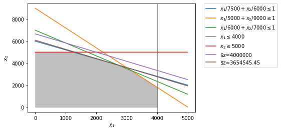
Using Python, we can represent the feasibility region:
[16]:
import numpy as np
import matplotlib.pyplot as plt
%matplotlib inline

x = np.linspace(0, 5000, 10000)
y1 = (1 - (x/7500))*6000
y2 = (1 -(x/5000))*9000
y3 = (1-(x/6000))*7000
y4 = 5000 + x*0
y5 = 0 + x*0

y9 = (4000000 - 500*x)/600
y10 = (3654545.45 - 500*x)/600

plt.plot(x, y1, label=r'$x_{1}/7500 + x_{2}/6000 \leq 1$')
plt.plot(x, y2, label=r'$x_{1}/5000 + x_{2}/9000 \leq 1$')
plt.plot(x, y3, label=r'$x_{1}/6000 + x_{2}/7000 \leq 1$')
plt.axvline(x=4000, label=r'$x_{1} \leq 4000$', color='grey')
plt.plot(x, y4, label=r'$x_{2} \leq 5000$')
plt.plot(x, y9, label=r'$z=4000000')
plt.plot(x, y10, label=r'$z=3654545.45')

y6 = np.minimum(y4,y1)
y7 = np.minimum(y6,y3)
y8 = np.minimum(y7, y2)

plt.fill_between(x, y8, y5, where=x <= 4000, color='grey', alpha=0.5)
plt.xlabel(r'$x_{1}$')
plt.ylabel(r'$x_{2}$')

plt.legend(bbox_to_anchor=(1.05,1), loc=2, borderaxespad=0. )
[16]:
<matplotlib.legend.Legend at 0x27dda19dec8>
Solution
When we display the objective function, we find out there are two candidates for the solution, one on the limit for \(x_{2}\) and the metal machining constraint. We can obtain the value of \(x_{1}\) and \(x_{2}\) at this point:
\(x_{2} = 5000\)
\(x_{1} = 7500*(1-x_{2}/6000)\)
\(z = 500*1250+600*5000 = 3006250\)
The other point represents the intersection between the metal machining constraint and the electric work constraint:
\((1-x_{1}/7500)*6000 = (1-x_{1}/6000)*7000\)
\(x_{1} = (7000-6000)/(7/6-6/7.5) = 2727.27\)
$x_{2} = 3818.18 $
\(z = 500*2727.27+600*3818.18 = 3654545.45\)
The second candidate provides a higher value and therefore is the optimal solution